2026 · Data engineering
Prototypisches Dashboard Luxemburger Verkehrsdaten
How I turned Luxembourg’s live traffic feeds into a history I could explore.
23 Jul–3 Sep 2026
Archived evaluation dataset
Inside the engineering
From a live feed
to a useful answer.
The CITA feeds showed current road conditions. I wanted a history I could query: what changes across hours, roads, and days? I built the collector and dashboard to find out.
Open a stage to inspect the decision.
Collect · PythonArchive before parsing.Live responses → preserved source
My collector runs as its own process. It saves each new response before parsing and uses SHA-256 hashes to detect duplicates.
The archive preserves what arrived. An interruption still leaves a gap in what I can analyse.
Read about the 18-hour gapStore · PostgreSQL 17Give the data its own history.Parsed responses → normalized measurements
I write normalized records to PostgreSQL. The dashboard reads this stored history independently of the live feeds.
I can compare roads, hours, and days without asking the source for those observations again.
2.8M measurements · 23 Jul–3 Sep 2026
Explore · Streamlit + PolarsMake the pattern inspectable.Stored history → hourly comparison
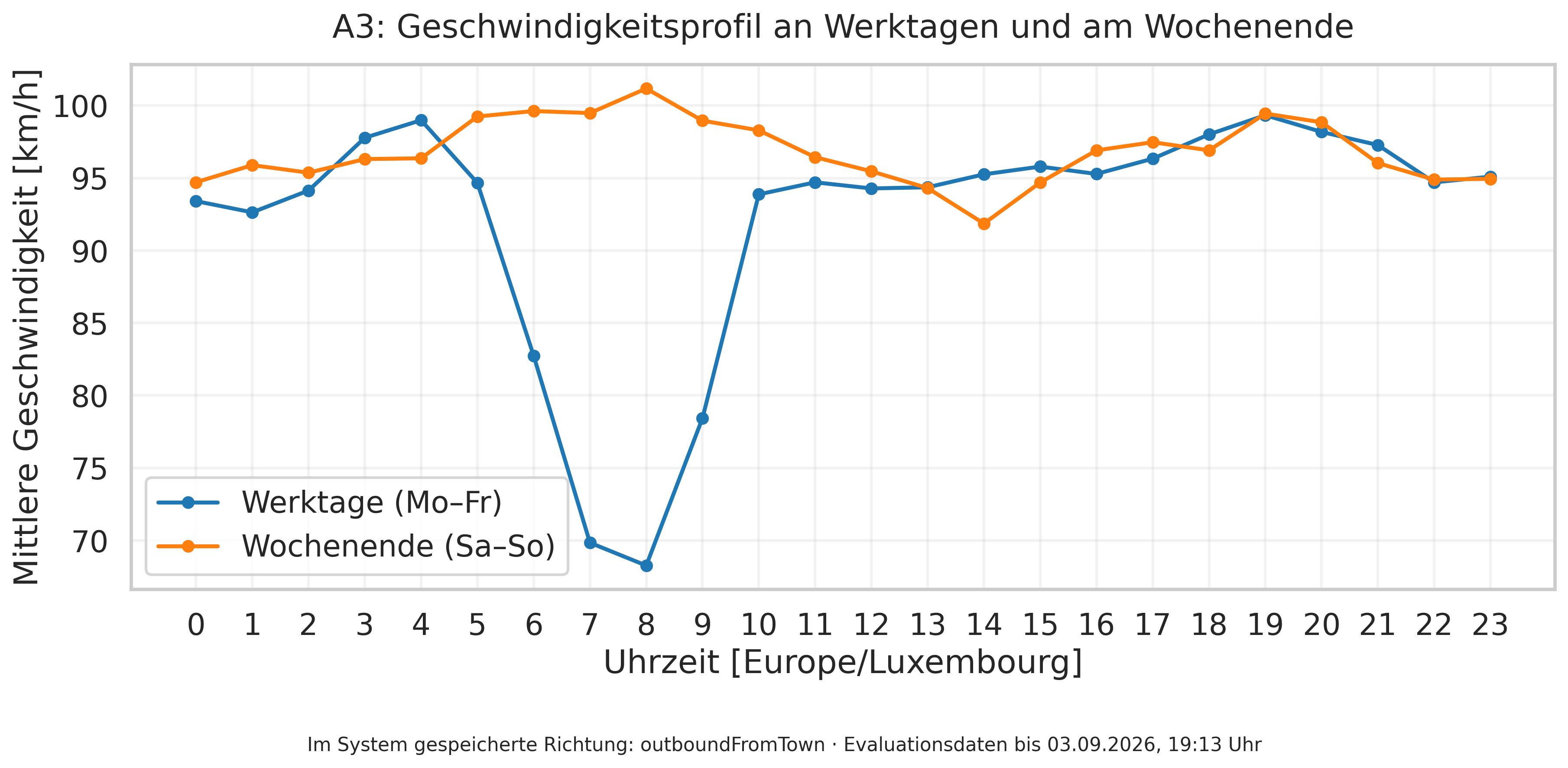
Polars prepares the analysis; my Streamlit dashboard queries the history. One finding was a weekday morning speed dip on the A3.
The figure below exposes the hourly means, observation counts, source window, and method.
Explore the A3 comparisonFrom my bachelor’s thesis
The A3, hour by hour.
In my sample, weekday speeds dipped in the morning; the weekend profile stayed steadier.
Weekday vs. weekend mean speeds · A3 · stored direction outboundFromTown
Explore the day Hover or drag to inspect an hour. Keyboard: ← / →, Home / End; Escape resets to 08:00.
I built the collector and dashboard so I could turn live traffic feeds into a history of patterns I could compare across hours and days.
Read the data and method
Source: my bachelor’s thesis, section 6.4.1 / figure 6.4, and its evaluation_hourly_profile.csv export. I grouped Monday–Friday and Saturday–Sunday and weighted each weekday/hour mean by its observation count, following the thesis plotting code. Source rows include positive speed, flow, and occupancy values; results are rounded to 0.1 km/h. The source window runs from 23 July 2026, 16:23 to 3 September 2026, 19:13 (Europe/Luxembourg).
View the 48-point aggregate JSON ↗ View the original thesis figure ↗
Scroll within the table to see all hours and columns. Speeds are in km/h; observation columns show sample counts.
| Hour | Weekday km/h | Observations | Weekend km/h | Observations |
|---|---|---|---|---|
| 00:00 | 93.4 | 4,357 | 94.7 | 1,731 |
| 01:00 | 92.6 | 4,236 | 95.9 | 1,730 |
| 02:00 | 94.1 | 4,217 | 95.4 | 1,651 |
| 03:00 | 97.8 | 4,334 | 96.3 | 1,644 |
| 04:00 | 99.0 | 4,404 | 96.4 | 1,632 |
| 05:00 | 94.7 | 4,503 | 99.2 | 1,641 |
| 06:00 | 82.7 | 4,502 | 99.6 | 1,645 |
| 07:00 | 69.8 | 4,580 | 99.5 | 1,675 |
| 08:00 | 68.3 | 4,600 | 101.2 | 1,706 |
| 09:00 | 78.4 | 4,559 | 99.0 | 1,645 |
| 10:00 | 93.9 | 4,540 | 98.3 | 1,682 |
| 11:00 | 94.7 | 4,531 | 96.4 | 1,699 |
| 12:00 | 94.3 | 4,611 | 95.5 | 1,726 |
| 13:00 | 94.4 | 4,543 | 94.3 | 1,693 |
| 14:00 | 95.3 | 4,578 | 91.9 | 1,671 |
| 15:00 | 95.8 | 4,581 | 94.7 | 1,685 |
| 16:00 | 95.3 | 4,614 | 96.9 | 1,669 |
| 17:00 | 96.3 | 4,680 | 97.5 | 1,702 |
| 18:00 | 98.0 | 4,685 | 96.9 | 1,662 |
| 19:00 | 99.3 | 4,500 | 99.4 | 1,659 |
| 20:00 | 98.2 | 4,460 | 98.8 | 1,732 |
| 21:00 | 97.3 | 4,441 | 96.0 | 1,751 |
| 22:00 | 94.7 | 4,364 | 94.9 | 1,749 |
| 23:00 | 95.1 | 4,405 | 94.9 | 1,697 |
On 25 July, a TLS negotiation failure left an 18-hour gap. I fixed collection, but couldn’t recover the missing measurements from the source. I learned to make gaps visible alongside the charts, rather than let a neat line imply the data was complete.